Why variational autoencoders?

Variational inference, and in particular its application to variational autoencoders (VAEs; Kingma & Welling, 2013; Rezende et al. 2014), is a powerful tool for learning to approximate complex probability distributions from data. However, the way it is often introduced initially made it seem somewhat mystical to me. In this post, I will try to introduce variational inference in a way that shows how it might arise from first principles as a natural solution to learning a neural-network-based latent-variable model. I will also highlight some of the nuances and subtleties that are often glossed over and motivate why we might want to learn a latent-variable model in the first place compared to other alternatives. This post will be a bit technical and assumes some familiarity with probability theory and machine learning.

As I have a background in reinforcement learning, I am particularly interested in how variational inference can be used to learn world models of the form $p(s^{\prime }\mid s,a)$. That is the probability of transitioning to state $s^{\prime }$ if an agent starts in state $s$ and takes action $a$. To abstract away from this specific use case I will just say we are interested in learning a distribution of the form $p(y\mid x)$. A non-reinforcement-learning example could be learning the distribution of images of digits conditional on the particular digit from 0 to 9 the image represents. Often variational inference is introduced as approximating the unconditioned distribution of a single variable $p(y)$, for example, the distribution of images of digits without conditioning on a particular digit. This is the difference between a conditional VAE (Sohn et al., 2015) and a standard VAE. In practice, this difference basically just involves an extra input to the neural network representing the conditioning variable, so it won’t add much complexity to the discussion.

Before getting into variational inference specifically, it’s worth unpacking what we mean by learning a distribution $p(y\mid x)$. This could mean a number of different things, in particular, we can distinguish at least three different types of models of $p(y\mid x)$ we might like to learn which are outlined in the textbook Reinforcement Learning: An Introduction by Sutton and Barto (2020):

• Sample Model: A model that takes in $x$ as input and stochastically outputs a single sample $y$ with approximately the same distribution as $p(y\mid x)$.
• Expectation Model: A model that takes in $x$ and outputs an estimate of $\mathbb{E}[y\mid x]$.
• Distribution Model: A model that takes in $x$ as input and outputs some representation of a distribution $\hat{p}(y\mid x)$ approximating the full distribution $p(y\mid x)$. For example, if $y$ is represented as a vector of binary variables, our model could output a vector of values between 0 and 1 representing the probability of each element of $y$ being 1 for that particular $x$.

The above definition of a distribution model is somewhat underspecified as I haven’t said how the distribution should be represented (do we have a closed-form expression? Does it suffice to be able to evaluate the probability of any $y$? If so how computationally expensive is this evaluation?). Nonetheless, this is a good starting point for a taxonomy of different types of models. Next, I’ll discuss some potential issues with learning expectation or distribution models before moving on to how latent-variable models can help address these issues.

Expectation models and distribution models

Given a dataset of $N$ samples $(x_i,y_i)$ indexed by $i\in \{0,1,..,N-1\}$, we can consider how each of these model types might be implemented and learned. For concreteness, let’s focus on the problem of modelling binary images of digits $y$ given the category $x\in \{0,...,9\}$. For an expectation model, we can just implement our model as a neural network represented by $f$ which outputs a vector of values between zero and one with one element for every pixel in the image.¹ Let $f(x_i;\theta )$ be the output of the neural network with parameters $\theta$ when given $x_i$ as input.² We can train this model by minimizing the pixel-wise mean squared error between the output of the network and the vector $y_i$ corresponding to the pixels of the actual image, that is we can minimize the following loss:

$$\mathcal{L}=\sum _{i=0}^{N-1}\Vert f(x_i;\theta )-y_i{\Vert }_2^2.$$

It’s straightforward to show that this loss is minimized when $f(x_i;\theta )$ outputs the mean over the dataset of $y_i$ associated with each $x_i$ which is exactly what we want for an expectation model. However, the expectation is obviously a very limited summary of the distribution. For example, if we give this model $x=9$ as input, the output will just be a blurry mashup of all the 9s in the dataset. For many downstream tasks, we will want more than this.

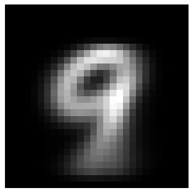
Image of the mean 9 from a binary version of MNIST, actually surprisingly recognizable as a 9.

If instead, we want to learn a distribution model, we have to decide on how we are going to represent the distribution. One simple choice is to take the same neural network $f$, but in this case, interpret the output $f(x_i;\theta )$ as the probability that each pixel is 1. We can then express the estimated probability of any image $y_i$ given a category $x_i$ as

$$\hat{p}(y_i\mid x_i;\theta )=\prod _j\{\begin{array}{ll}f(x_i;\theta )[j]& \text{ if }{y}_i[j]=1\\ 1-f(x_i;\theta )[j]& \text{ if }{y}_i[j]=0,\end{array}$$

where I’ve used the square bracket notation to index individual elements of a vector, whereas subscripts index dataset elements. We can then train this model by maximizing the log-likelihood of the data under the model, that is we can minimize the following loss:

$$\begin{array}{}\text{(1)}& \mathcal{L}=-\sum _{i=0}^{N-1}\log (\hat{p}(y_i\mid x_i;\theta )).,\end{array}$$

which is the negation of the log-likelihood of the data under our model. If we assume our data is drawn from some underlying distribution $p(y,x)=p(y\mid x)p(x)$, then minimizing this loss is equivalent to minimizing an unbiased estimate of the expectation over $x$ of the KL divergence between $p(y\mid x)$ and $\hat{p}(y\mid x;\theta )$, that is

$$\begin{gathered} {\mathbb{E}}_x[KL(p(y|x),\hat{p}(y|x))] \\ ={\int }_{x,y}p(x)(p(y|x)(\log (p(y|x))-\log (\hat{p}(y|x;\theta ))), \end{gathered}$$

note that the first term in the integrand does not depend on $\theta$ and thus does not affect the optimization. KL divergence is always nonnegative, and zero if and only if the two distributions match exactly. It also has intriguing interpretations in terms of the expected number of extra bits required to encode samples from one distribution using a code optimized for the other.³ Furthermore, we can often bound the utility of the model for downstream applications in terms of the KL divergence between the true distribution and the model distribution. For example, in reinforcement learning, we can bound the expected detriment in return we suffer by optimizing a policy for a learned model instead of the true model in terms of the KL divergence between the two (Ross & Bagnell, 2012). In this sense, KL divergence is a reasonable objective for model learning, though certainly not the only possible objective.

In the specific case where we are dealing with binary vectors, the minima of Equation $\text{(1)}$ is actually the same as the minima of the mean squared error loss we used for the expectation model.⁴ Likewise, the resulting model is not much more useful. While technically, we are now representing a distribution, it is a distribution of a specific limited form. In particular, since we represent the probability of each pixel being one independently, we can’t represent any correlations between pixels. If we sample a particular 9 from the distribution represented by this model it might loosely resemble a 9 but with scattered dots rather than smooth connected lines as each pixel will be sampled as if it belonged to a different 9.

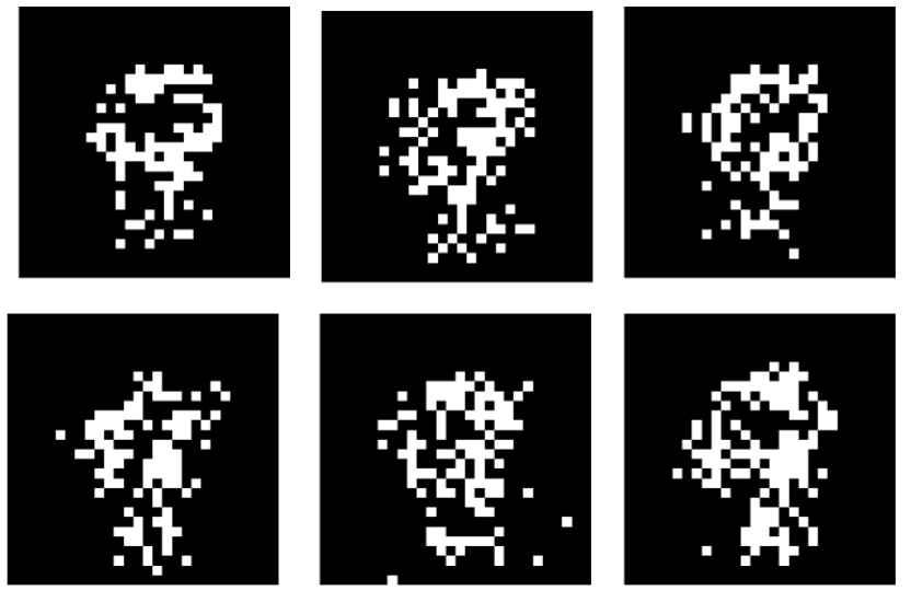
Images sampled according to independent pixel probabilities across all 9s.

At this point, we could try to improve our distribution model by making it more expressive. However, if we are committed to outputting some representation of the full conditional distribution in closed form, this will probably be an uphill battle. The most general distribution over binary images is a vector of probabilities for each possible image, $2^{28\times 28}\approx {10}^{236}$ elements for a 28x28 image. Clearly, we don’t want to output a vector of this size, so we would have to make some trade-off between generality and simplicity in the form of our output distribution. We could spend some time thinking about various restricted distributions that might do a good job of representing reasonable images. Alternatively, we could give up on trying to output a closed-form expression for the full distribution and instead try to learn something like a sample model.

If we give up on representing a closed-form expression for the distribution, it’s no longer clear whether we can optimize our model by simply minimizing the loss in Equation $\text{(1)}$. Doing so requires us to evaluate, and differentiate $\hat{p}(y_i\mid x_i;\theta )$ which we can’t do if all our model gives is samples from the distribution. In the next section, I will discuss autoregressive models which are sort of an intermediate between distribution models and sample models in the sense that they don’t represent the full distribution in any closed form, but we can still efficiently evaluate the probability of any $y$ for a given input $x$ under the model.

Autoregressive models

For an autoregressive model, we assume each $y$ consists of $M$ features such that $y=(y[0],...y[M-1])$. In our running digits example this could just be the pixels of the image. Rather than approximating the full joint distribution of $y$, an autoregressive model learns approximate conditional distributions for each feature $\hat{p}(y[i]\mid y[0],...,y[i-1],x;\theta )$. There is an implicit assumption that the individual features have a simple enough form that we can explicitly represent their distribution in closed form (e.g. a vector of probabilities for each of a finite set of values). In our running example, we could represent the probability of each pixel being one as a Bernoulli variable.

Example of an image of a 9 being generated by an autoregressive process, each pixel is sampled with probability that depends on the pixels generated so far. In principle, arbitrary distributions over binary images can be represented in this form.

Given an autoregressive model, we can sample $y$ by sampling from each conditional distribution sequentially. It is possible to represent arbitrary distributions in this autoregressive form.⁵ Furthermore, in this case we can evaluate $\hat{p}(y\mid x;\theta )=\prod _{i=0}^{M-1}\hat{p}(y[i]\mid y[0],...,y[i-1],x;\theta )$ for arbitrary $y$. Thus with an autoregressive model, we can optimize the loss in Equation $\text{(1)}$. Although sampling must be done sequentially, evaluation of the probability of a particular $y$ can be done for all features in parallel. This is crucial for efficient training of large language models (LLMs) for example.

Although autoregressive models are popular, for example in LLMs, they have some notable drawbacks. They require features to be sampled sequentially, limiting the potential for parallelism in sampling. They also require a choice of closed-form distribution to model the individual factors which may be limiting, for example, if the individual factors can take continuous values. One could commit to a particular choice of distribution, such as a Gaussian, but this would again limit the representation power of the model, as it could not represent multimodal conditional distributions for individual features. Finally, autoregressive models require a, potentially arbitrary, choice of the order in which features are sampled, which can be unnatural and may result in complicated conditional distributions that are difficult to model. For example, consider the challenge of autoregressively modelling the distribution of pixels in a complex image in arbitrary order.

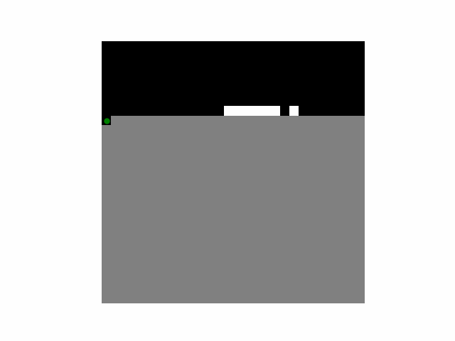
To drive home the last point, one can even construct distributions where an autoregressive model faces fundamental computational challenges in representing the conditional distributions while representing the joint distribution of features is easy. For example, imagine a process which first selects a uniform random integer $y_1$ and then generates $y_2=g(y_1)$ using some function $g$ which is easy to compute but difficult to invert.⁶ Now imagine we want to model $p(y_2{y}_1)$ where $y_2{y}_1$ represents the sequence of bits in the integers $y_2$ and $y_1$ concatenated together. A bitwise autoregressive model of $p(y_2{y}_1)$ would have to first generate a random output $y_2$, and then invert $g$ in order to accurately model $p(y_1\mid y_2)$. On the other hand, a more general model that samples from the joint distribution as a whole would be free to simulate sampling $y_1$ followed by computing $y_2=g(y_1)$, which is easy. See the work of Lin et al. (2020) for a more detailed discussion of some related issues with autoregressive models.⁷

Example highlighting how autoregressive modeling can be fundamentally more difficult than modeling the full joint distribution of features. The original process being modeled uses a one-way function. An autoregressive model operating in the reverse order is forced to invert the function to accurately capture the conditional distribution.

Latent-variable models

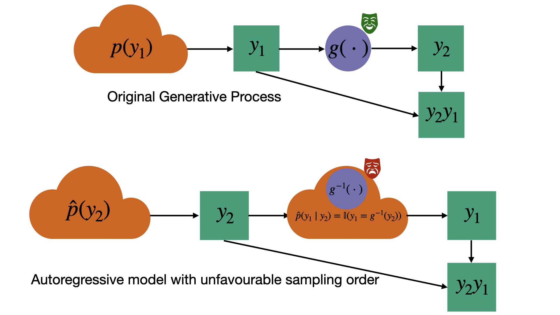
Another class of sample models, which can help to address the challenges outlined so far, is called latent-variable models. The basic idea is to factor the nontrivial part of the randomness in our learned distribution into a separate noise variable $z$, generally referred to as the latent variable. We then use a latent-variable-dependent distribution $\hat{p}(y\mid x,z;\theta )$ to model the distribution of $y$ given $z$ and $x$.

Normally, $\hat{p}(y\mid x,z;\theta )$ has a simple closed form as a function of $y$. For example, if $y$ is a vector of binary variables, $\hat{p}(y\mid x,z;\theta )$ could simply be a neural network which takes $x$ and $z$ as input and outputs the mean of each element of $y$. Note that this means the elements of $y$ are uncorrelated given $z$. The latent variable $z$ itself will also be drawn from a simple closed form prior distribution $\hat{p}(z\mid x;\theta )$ conditioned on the input $x$.⁸ For example, $\hat{p}(z\mid x;\theta )$ could also be represented as a neural network which takes $x$ as input and outputs the mean of each element of $z$, where each element of $z$ is once again a Bernoulli variable. I will use vectors of Bernoulli variables as a running example in what follows but other choices, such as vectors of independent Gaussians or categorical variables, are possible and common.

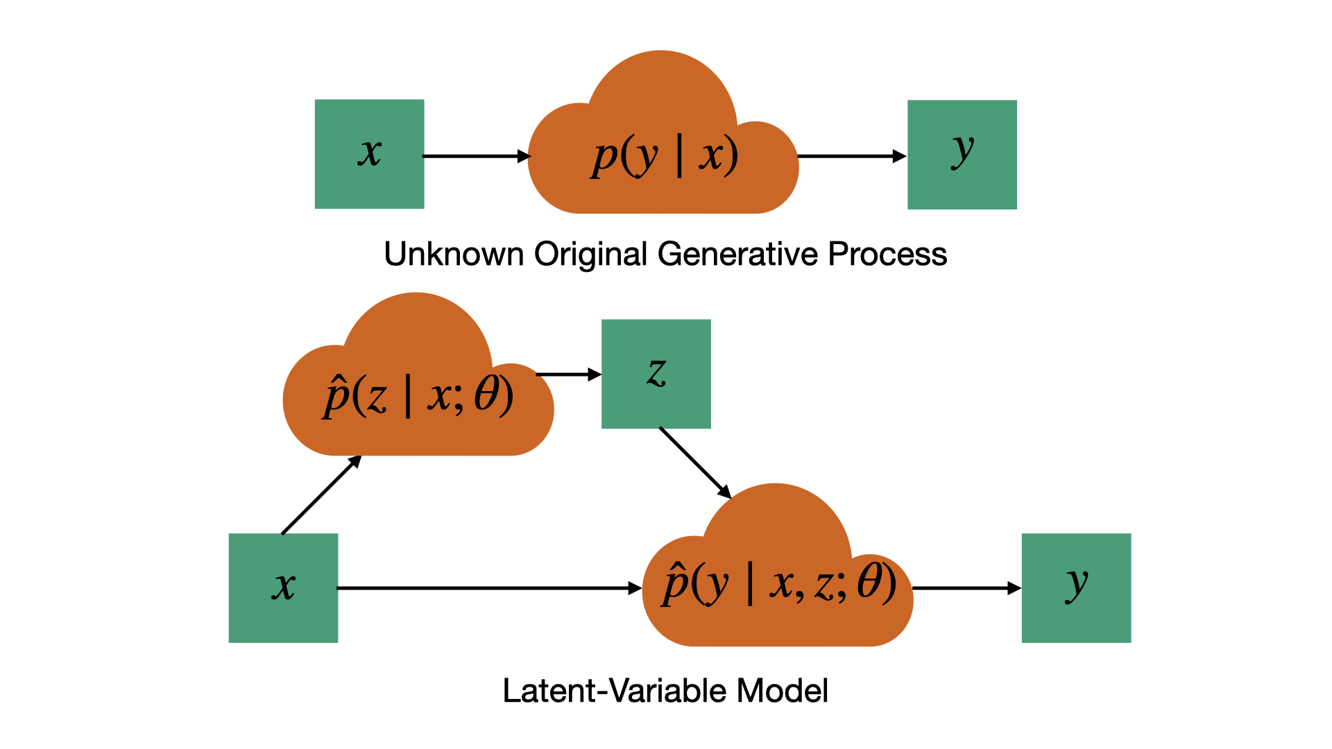
Illustration of sampling process for a latent-variable model. Rather than modeling the distribution of y conditioned on x directly we first sample a latent-variable z, and then sample y conditioned on both x and z. This allows representation of complex distributions of y conditioned on x despite the distributions of z conditioned on x, and y conditioned on x and z having a simple closed-form. The price we pay for this representational power is that we can no longer easily evaluate or optimize the likelihood of the data under our model.

Since the mapping $\hat{p}(y\mid x,z;\theta )$ is parameterized by a generic neural network capable of representing complex transformations $\hat{p}(y\mid x;\theta )={\int }_z\hat{p}(y\mid x,z;\theta )\hat{p}(z\mid x;\theta )$ can capture complicated dependencies between elements of $y$ despite $\hat{p}(y\mid x,z;\theta )$ and $\hat{p}(z\mid x;\theta )$ being simple factored distributions. In order to draw a sampled $y$ from this model, we sample $z\sim \hat{p}(z\mid x;\theta )$ first, then compute $\hat{p}(y\mid x,z;\theta )$, and finally sample $y\sim \hat{p}(y\mid x,z;\theta )$. The basic idea here is quite natural, we wish to represent a potentially complex distribution, and we know that neural networks are universal function approximators, so we can use the neural network to map an arbitrary, sufficiently rich, noise variable $z$ to a sample from the distribution we wish to represent.

The next question is: how do we train a latent-variable model from data? We’d like to optimize $\hat{p}(y\mid x;\theta )$ with respect to the loss in Equation $\text{(1)}$, however, just evaluating $\log (\hat{p}(y\mid x;\theta ))$ in this case requires us to integrate over $z$ which in the case where $z$ is a vector of Bernoulli variables means summing over combinatorially many values. We want $z$ to be large enough to capture fairly general dependence among the elements of $y$, in which case explicit integration will usually be intractable. The price we have paid for the generality of using a neural network to model the complexity of the distribution is that we can no longer straightforwardly compute or optimize the log-likelihood of the data under our model. This is where the idea of variational inference comes in.

Variational inference

Computing $\hat{p}(y\mid x;\theta )$ requires an intractable integration over $z$, but computing $\hat{p}(y\mid x,z;\theta )$ is fairly easy, it’s just a forward pass through a neural network. If we imagine the ground truth distribution was also generated by first sampling $z$, and we could observe the $z$ associated with each sample, we could minimize an empirical estimate of $KL(p(y,z\mid x),\hat{p}(y\mid x,z;\theta )\hat{p}(z\mid x;\theta ))$, equivalent to minimizing the following loss:

$$\begin{array}{rl}\mathcal{L}& =\sum _{i=0}^{N-1}\log (p(y_i^{\prime },z_i\mid x_i))-\log (\hat{p}(y_i^{\prime }\mid x_i,z_i;\theta )\hat{p}(z_i\mid x_i;\theta ))\\ & =\sum _{i=0}^{N-1}\log (p(y_i^{\prime },z_i\mid x_i))-\log (\hat{p}(y_i^{\prime }\mid x_i,z_i;\theta ))-\log (\hat{p}(z_i\mid x_i;\theta ))\\ & \propto -\sum _{i=0}^{N-1}\log (\hat{p}(y_i^{\prime }\mid x_i,z_i;\theta ))+\log (\hat{p}(z_i\mid x_i;\theta )),\end{array}$$

where $z_i$ is the observable latent variable associated with each sample and, in the final line, I’ve dropped a term which does not depend on $\theta$. This is a stronger requirement than only matching the distributions with respect to $y$. If we manage to make $KL(p(y,z\mid x),\hat{p}(y\mid x,z;\theta )\hat{p}(z\mid x;\theta ))=0$ this also guarantees $KL(p(y\mid x),\hat{p}(y\mid x;\theta ))=0$ since if the joint distributions over $y,z$ are the same then logically the marginal distribution over $y$ must also be the same.

Unfortunately, there is no reason to believe the true distribution is actually generated by first sampling a latent variable $z$, and even if it was, this latent variable is certainly not observable as required by the above objective. Variational inference works around this issue by augmenting the true distribution with an approximate posterior distribution over $z$, $\hat{q}(z\mid x,y;\theta )$. Intuitively speaking, we ask: if the actual data was generated by first sampling a latent variable $z$, just like in our model, what is the distribution of $z$ values that could have generated the observed $y$ given the observed $x$?

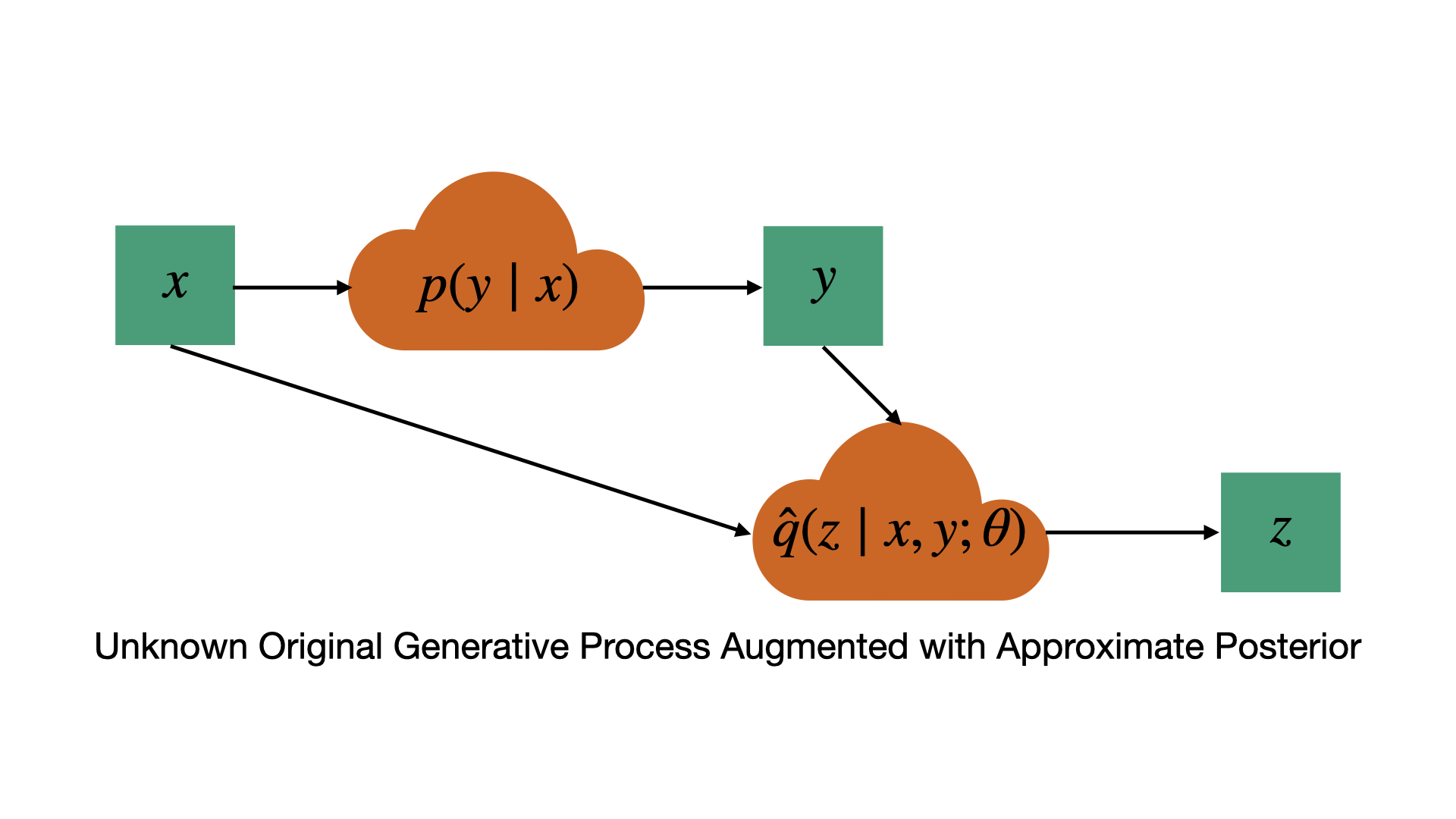
The unknown original generative process from which the data arose, augmented with an approximate posterior. With the addition of the approximate posterior, this process now generates samples in the joint space of y and z, just like our generative model. Unlike the probability of y alone, we can directly evaluate the joint probability of y and z under our generative model, so we can consider performing maximum likelihood in the joint space.

I see this as the essential idea behind variational inference so it’s worth reiterating. We have a generative model for some variable $y$ which generates samples using an intermediate latent variable $z$ and we’d like to train this model to generate samples that match the distribution of the data. If the data also included a latent variable $z$, we could essentially do this by maximum likelihood of the joint distribution over $y$ and $z$. However, the data does not include such a latent variable so instead we augment the data distribution with a conditional distribution $\hat{q}(z\mid x,y;\theta )$ over $z$. Together with the true distribution $p(y\mid x)$ from which the data was sampled, this leads to a joint distribution $p(y,z\mid x)=p(y\mid x)\hat{q}(z\mid x,y;\theta )$ which we can now use as a target distribution for our model. The part of this story that takes a bit of effort to grok, at least for me, is that it doesn’t matter that the true distribution was not generated by first sampling $z$, we can still optimize the joint KL divergence between the true distribution, augmented with an approximate posterior, and our model distribution. Next, I will explain how this is done more precisely.

Often the approximate posterior $\hat{q}(z\mid x,y;\theta )$ is parameterized as a neural network which outputs a distribution with the same form as $\hat{p}(z\mid x;\theta )$. If $\hat{p}(z\mid x;\theta )$ is a vector of uniform Bernoulli variables, $\hat{q}(z\mid x,y;\theta )$ could be parameterized as an equal length vector of Bernoulli variables with means output by a neural network, which now takes both $x$ and $y$ as input. We can now consider minimizing an empirical approximation to $KL(\hat{q}(z\mid x,y;\theta )p(y\mid x),\hat{p}(y\mid x,z;\theta )\hat{p}(z\mid x;\theta ))$, let’s start by expanding as follows:

$$\begin{array}{rl}KL& (\hat{q}(z\mid x,y;\theta )p(y\mid x),\hat{p}(y\mid x,z;\theta )\hat{p}(z\mid x;\theta ))\\ & ={\mathbb{E}}_{x,y,z}[\log (\hat{q}(z\mid x,y;\theta )p(y\mid x))-\log (\hat{p}(y\mid x,z;\theta )\hat{p}(z\mid x;\theta ))]\\ & \propto {\mathbb{E}}_{x,y,z}[\log (\hat{q}(z\mid x,y;\theta ))-\log (\hat{p}(y\mid x,z;\theta ))-log(\hat{p}(z\mid x;\theta ))]\\ \text{(2)}& & ={\mathbb{E}}_{x,y}[{\mathbb{E}}_{z\sim \hat{q}(z\mid x,y;\theta )}[\log (\hat{q}(z\mid x,y;\theta ))-\log (\hat{p}(y\mid x,z;\theta ))-\log (\hat{p}(z\mid x;\theta ))]].\end{array}$$

Note that, in the second last line, I have dropped the term ${\mathbb{E}}_{x,y,z}[\log (p(y\mid x))]$ which does not depend on $\theta$ and thus is not relevant to its optimization. Importantly, we optimize Equation $\text{(2)}$ with respect to all the parameters of $\hat{q}(z\mid x,y;\theta )$ and $\hat{p}(y\mid x,z;\theta )$ and $\hat{p}(z\mid x;\theta )$, not just the parameters of $\hat{p}(y\mid x,z;\theta )$ as we did in Equation $\text{(1)}$. The final expression in Equation $\text{(2)}$ is an expectation over the data distribution of another expectation involving some functions we can evaluate in closed form. It’s starting to look like something we can actually optimize, but I’ll defer the question of how precisely to do it until a little later. First, let’s think about whether this is a reasonable thing to do.

Is this a reasonable thing to do?

Even though we are using a learned distribution $\hat{q}(z\mid x,y;\theta )$ instead of some ground truth distribution over $z$, we can still say that if we managed to reduce $KL(\hat{q}(z\mid x,y;\theta )p(y\mid x),\hat{p}(y\mid x,z;\theta )\hat{p}(z\mid x;\theta ))$ to zero for all $x$ this will suffice to ensure that $KL(p(y\mid x),\hat{p}(y\mid x;\theta ))$ is zero as well, and thus our model matches the data distribution. In fact, we can actually make a stronger statement than this. In particular, KL divergence is additive in the following sense:

$$\begin{array}{rl}KL(p(y\mid x)p(x),q(y\mid x)q(x))& =KL(p(x),q(x))+{\mathbb{E}}_x[KL(p(y\mid x),q(y\mid x)]\\ & \ge KL(p(x),q(x)).\end{array}$$

In our situation, this gives

$$KL(\hat{q}(z\mid x,y;\theta )p(y\mid x),\hat{p}(y\mid x,z;\theta )\hat{p}(z\mid x;\theta ))\ge KL(p(y\mid x),\hat{p}(y\mid x;\theta )).$$

Thus, by minimizing the left-hand side we are minimizing an upper bound on the right-hand side. In other words, however low we can make the left-hand side, we can guarantee the right-hand side is even lower. For this reason the (negation of the) inner expectation in Equation $\text{(2)}$ is often called the Evidence Lower Bound (ELBO).

But why should we believe it’s even possible to achieve $KL(\hat{q}(z\mid x,y;\theta )p(y\mid x),\hat{p}(y\mid x,z;\theta )\hat{p}(z\mid x;\theta ))$ close to zero given our restrictive choice of approximate posterior? A particular choice of $\hat{p}(y\mid x,z;\theta )$ and $\hat{p}(z\mid x;\theta )$ will correspond to a certain posterior over $z$ which we can work out using Bayes theorem:

$$\hat{p}(z\mid x,y;\theta )=\frac{\hat{p}(y\mid x,z;\theta )\cdot \hat{p}(z\mid x;\theta )}{\int \hat{p}(y\mid x,z;\theta )\cdot \hat{p}(z\mid x;\theta )dz}.$$

To push the KL divergence to zero we would require $\hat{p}(z\mid x,y;\theta )=\hat{q}(z\mid x,y;\theta )$. Unfortunately, this posterior need not have the factored form we imposed on $\hat{q}(z\mid x,y;\theta )$, i.e. there may be correlation among the different elements of $z$. The situation is improved a bit by noting that there need not be one unique $\hat{p}(y\mid x,z;\theta )$ which minimizes $KL(p(y\mid x),\hat{p}(y\mid x;\theta ))$, there may be many ways to map the latent variable $z$ to $y$ such that our sample model captures the true distribution.

If there exists some mapping $\hat{p}(y\mid x,z;\theta )$ that captures $p(y\mid x)$ when we marginalize out $z$ while also leading to a factored posterior $\hat{p}(z\mid x,y;\theta )$, then that solution will be preferred in terms of Equation $\text{(2)}$. But do such solutions even exist? In general, not necessarily, but for sufficiently expressive neural networks, along with a sufficiently rich $z$, it will be possible to make the KL arbitrarily small. This is essentially analogous to a universal approximation theorem for VAEs, which I will next demonstrate holds, at least for the case of Bernoulli vectors.

If we consider the case where all relevant distributions are Bernoullis, then $y$ can take finitely many possible values. In particular, if $y$ is a binary vector of length $n$, then $y$ can take $N=2^n$ distinct values. Let’s index these possible values as $y_0,...,y_{N-1}$. For realistic data, it is likely that the vast majority of these values will have near zero probability under the true distribution $p(y\mid x)$ so the effective $N$ could be much smaller. Now consider the extreme case where $z$ is a vector of $N$ independent Bernoulli variables. We can then associate each possible value of $y$ with an element of $z$ by choosing

$$\hat{p}(y_i\mid x,z;\theta )=\prod _{j=0}^{i-1}\mathbb{I}(z[j]=0)\mathbb{I}(z[i]=1)$$

where $\mathbb{I}$ is the indicator function. In words, we deterministically map each $z$ to the $y_i$ corresponding to the index of the first 1 in $z$.⁹ We can then set $\hat{p}(z\mid x;\theta )$ such that

$$p(y_i\mid x)=\prod _{j=0}^{i-1}\hat{p}(z[j]=0\mid x;\theta )\hat{p}(z[i]=1\mid x;\theta ),$$

which ensures that $\hat{p}(y_i\mid x;\theta )=p(y_i\mid x)$ for all $i$. Furthermore, the true posterior will factor as

$$\hat{p}(z\mid y_i,x;\theta )=\prod _{j=0}^{i-1}\mathbb{I}(z[j]=0)\mathbb{I}(z[i]=1)\prod _{j=i+1}^{N-1}\hat{p}(z[j]\mid x;\theta ),$$

and thus can be represented by a factored approximate posterior $\hat{q}(z\mid x,y_i;\theta )$. Intuitively, this just says that if we observe a particular $y_i$ generated by the above process, we know that the first $i-1$ elements of $z$ must have been zero, and the $i$th element must have been one, but we have no information about the remaining elements of $z$ beyond the prior. Note that this construction requires the prior $\hat{p}(z\mid x;\theta )$ to be parameterized and conditioned on $x$, it’s an interesting question whether an analogous construction is possible with a fixed prior $\hat{p}(z)$.

The above construction is not a very efficient way to utilize the elements of our latent variable, requiring a separate element for each possible outcome $y$. There is no doubt much more that could be said about the representational capabilities of latent-variable models trained with variational inference which is beyond the scope of this post, and I am not currently very knowledgeable of the relevant literature. It’s also worth noting that the existence of such solutions does not mean we can necessarily find them by stochastic gradient descent. Nevertheless, the construction presented here is a nice sanity check to show that the variational inference approach I’ve described is capable of modelling arbitrary distributions in principle, at least in the Bernoulli case. I encourage the interested reader to think about how one could utilize the latent variable more efficiently while still maintaining the factored posterior, as well as how one could define similar constructions for other types of latent variable such as vectors of independent Gaussians.

Optimizing the ELBO

Now let’s consider the question of how we can optimize Equation $\text{(2)}$. We will use stochastic samples of $x,y$ observed from the true unknown distribution, which takes care of the outer expectation, however, we still need to deal with the inner expectation. We cannot simply sample $z\sim \hat{q}(z\mid x,y;\theta )$ and optimize the inside of the expectation with respect to the samples as the sampling distribution itself depends on $\theta$. However, as long as we can evaluate, sample from, and differentiate $\hat{q}(z\mid x,y;\theta )$, which we guarantee by design, we can use the following general identity to obtain an unbiased gradient estimate:

$$\frac{\partial }{\partial \theta }{\mathbb{E}}_{z\sim q(z;\theta )}[f(z;\theta )]={\mathbb{E}}_{z\sim q(z;\theta )}[\frac{\partial \log (q(z;\theta ))}{\partial \theta }f(z;\theta )+\frac{\partial }{\partial \theta }f(z;\theta )].$$

In our case, we would take $q(z\mid \theta )=\hat{q}(z\mid x,y;\theta )$ and $f(z;\theta )=\log (\hat{q}(z\mid x,y;\theta )-\log (\hat{p}(y\mid x,z;\theta ))-\log (\hat{p}(z\mid x;\theta ))$. We can then derive an unbiased estimator of the gradient by sampling from $q(z;\theta )$ and optimizing the inside of the expectation for the specific sample. This estimator is nice in that it’s generic and unbiased, however, it can have high variance to the point that it’s usually not very practical. Luckily, in many situations, it is possible to derive lower variance unbiased gradient estimates such as the reparameterization trick (Kingma & Welling, 2013; Rezende et al. 2014) for continuous latent-variables. There are plenty of resources on the reparameterization trick, so I will not cover it here. Biased gradient estimators such as the straight-through estimator (Bengio et al., 2013) can also be used for discrete latent-variables and often perform well in practice.

Latent dynamics models for reinforcement learning

I have described how to train a basic (conditional) latent-variable model using variational inference. One could directly apply the described approach to learn a world model for reinforcement learning simply by replacing $x$ with the state-action pair $(s,a)$ and $y$ with the following state $s^{\prime }$ and having the latent variable $z$ represent the noise in the transition dynamics. Often, however, a slightly different setup is used. In particular, rather than using the latent variable only to parameterize transition noise, one can learn a mapping $\hat{p}(z\mid s;\theta )$ and then model the dynamics themselves in latent space as $\hat{p}(z^{\prime }\mid z,a;\theta )$. An additional learned distribution $\hat{p}(s^{\prime }\mid z^{\prime };\theta )$ aims to reconstruct the distribution of next states (see e.g. Watter et al. (2015), Ha and Schmidhuber (2018)). The overall transition distribution is then modelled as

$$\hat{p}(s^{\prime }\mid s,a)={\int }_{z,z^{\prime }}\hat{p}(z\mid s;\theta )\hat{p}(z^{\prime }\mid z,a;\theta )\hat{p}(s^{\prime }\mid z^{\prime };\theta ).$$

In this case, we are effectively trying to transform states $s$ into a new space in which the dynamics obey the factored structure imposed by $\hat{p}(z^{\prime }\mid z,a;\theta )$. This approach has a number of benefits including being able to roll out the model for multiple steps in latent space, without explicitly predicting the environment state in each step. This is essentially the approach of Dreamer (Hafner et. al. 2020; Hafner et. al. 2021; Hafner et. al. 2023) which has demonstrated impressive results for model-based reinforcement learning.

Closing thoughts

The application of variational inference to learn latent-variable models is a rich and active area of research. I have only scratched the surface of the topic here, but the principles presented should apply quite generally. For example, one may wish to use models which include different latent variables at various points in the generative process to capture more complex dynamics and relationships. In such cases, one can still think in terms of minimizing KL-divergence between our generative model and an augmented version of the data distribution which includes approximations to the distribution of each latent variable which is used by our generative model but does not appear in the data. I have found this way of thinking to be a very useful lense to understand what is happening when seeing a particular variational approach for the first time.

There are also a number of alternative techniques for learning probability distributions which strike different trade-offs in terms of ease of sampling, evaluating probabilities, and learning, many of which I have not discussed at all. Some examples include energy-based models, diffusion models, and flow-based models.

My aim in this post was to introduce the concept of variational inference for learning latent-variable models in a way that makes it seem more natural than the way in which I have usually seen it presented. I also emphasized some of the nuances, like the question of whether it’s even possible to make the ELBO arbitrarily small, which I personally consider interesting and important but which are often glossed over. I hope this overview can help others to more rapidly pick up some of the intuitions about variational inference that I have found useful, but which have taken me a long time to develop.

References

Bengio, Y., Léonard, N., & Courville, A. (2013). Estimating or propagating gradients through stochastic neurons for conditional computation. arXiv preprint arXiv:1308.3432.

Ha, D., & Schmidhuber, J. (2018). World models. Advances in Neural Information Processing Systems.

Hafner, D., Lillicrap, T., Ba, J., & Norouzi, M. (2020). Dream to control: Learning behaviors by latent imagination. International Conference on Learning Representations.

Hafner, D., Lillicrap, T. P., Norouzi, M., & Ba, J. (2021). Mastering atari with discrete world models. International Conference on Learning Representations.

Hafner, D., Pasukonis, J., Ba, J., & Lillicrap, T. (2023). Mastering diverse domains through world models. arXiv preprint arXiv:2301.04104.

Kingma, D. P., & Welling, M. (2014). Auto-encoding variational bayes. International Conference on Learning Representations.

Lin, C.-C., Jaech, A., Li, X., Gormley, M. R., & Eisner, J. (2020). Limitations of autoregressive models and their alternatives. arXiv preprint arXiv:2010.11939.

Rezende, D. J., Mohamed, S., & Wierstra, D. (2014). Stochastic backpropagation and approximate inference in deep generative models. International Conference on Machine Learning.

Ross, S., & Bagnell, J. A. (2012). Agnostic system identification for model-based reinforcement learning. International Conference on Machine Learning.

Sohn, K., Yan, X., & Lee, H. (2015). Learning structured output representation using deep conditional generative models. Advances in neural information processing systems.

Sutton, R. S., & Barto, A. G. (2020). Reinforcement learning: An introduction (second edition). MIT Press.

Watter, M., Springenberg, J., Boedecker, J., & Riedmiller, M. (2015). Embed to control: A locally linear latent dynamics model for control from raw images. Advances in neural information processing systems.

Footnotes

1. A neural network is really overkill here since the input simply takes one of 10 values, we would probably be better off just storing a separate vector of pixels for each digit. However, it’s easy to imagine how a neural network could be useful for handling more complex input such as a state-action pair in reinforcement learning. ↩

2. Throughout this post, I will use $\theta$ to represent an arbitrary set of all learnable parameters for simplicity. When dealing with multiple parameterized functions each function will usually only depend on a disjoint subset of all parameters. ↩

3. See, for example, this blog post for an excellent discussion of KL divergence and other information theoretic concepts. ↩

4. This is only true for an overparameterized neural network that can perfectly fit the data. For an underparameterized network, the two losses will differ in how they utilize the limited network capacity. ↩

5. As I mentioned previously, this is not possible with an approximation of the simpler form $\hat{p}(y[i]\mid x;\theta )$ as there is no way to capture correlation between features. ↩

6. More precisely, say $g(y_1)$ can be computed in polynomial time but $g^{-1}(y_2)$ cannot. While the existence of such functions technically remains an open question, much of modern cryptography relies on assuming they exist. ↩

7. Prompting techniques which give a LLM a chance to output some extra information before the answer (for example “Let’s think through this step by step…”) can provide one way to circumvent such limitations. In the above example, the model could commit to a particular $y_1$ and then predict $y_2=g(y_1)$ in its reasoning process before outputting the $y_2{y}_1$ as its final answer. ↩

8. One could also use a distribution $\hat{p}(z;\theta )$ which does not depend on $x$, or $\hat{p}(z)$ which is fixed instead of learned. These choices may however limit the representational power of the model as I will discuss shortly. ↩

9. If you’re reading very closely, you’ll notice I haven’t defined what happens when $z$ is all zeros, good catch! Really we only need $N-1$ elements of $z$ to represent $y$ and the all zero $z$ can be used to represent the last value of $y$. ↩